Styles (Mark from Styles Gallery) Display1 style removed ✓
1
1
1.3.2
Display2 style modified
Numbering added in format 1., 2., ✓ (Accept 1), 2),)
Any border added ✓
Left indent set to 0 cm ✓
All occurrences of the style updated ✓
1 1 1 1
4
1.4
Cross reference (Figure 3: Gourmet Meals)
Cross reference inserted within brackets ✓ (Accept hyperlink/ bookmark)
Reference to label 'Figure 3: Gourmet Meals' ✓
1 1
2
1.5
Language Word 'explore' language changed to English (South Africa) ✓ (mark from task bar)
1
1
1.6
Tabs
Tab set at 2 cm ✓
Left aligned ✓
Tab set at 10 cm ✓
Right aligned ✓
Solid leader tab set ✓
Tab settings applied to all lines ✓
1 1 1 1 1 1
6
1.7
Citation (Ward)
Citation to 'Jean Ward' source inserted ✓
Year does not display ✓
1 1
2
1.8.1
Caption (Figure 6: Jumping Castle) (Alt + F9)
Automatic figure caption added ✓ to correct picture
Text 'Jumping Castles' inserted ✓ for caption
1 1
2
1.8.2
Table of figures Table of figures updated ✓ (see 'Figure 5: Wine Shop')
1
1
1.9
Bibliography
Book, A. (2015). Too little too late. Entertainment All. Business To All. (2016, July). Retrieved from Biz Communities: www.biz_com.com Sousher, P. L. (2014). Marketing South Africa. Business Journal, 61-62.
Ward, J. (2005). Coetzenburg: A Tourist Site.
Automatic bibliography inserted ✓
Appears in APA style ✓
1 1
2
1.10
Page numbering and section numbering
Page number does not appear on first page ✓
Section 2/Last page formatted with i, ii, iii, … format ✓ starts from i ✓
Style of page number with 'i' not changed ✓
1 1 1 1
4
Total for QUESTION 1
[34]
QUESTION 2 File name: 2Stay Total Q2: 16
No.
Criteria
Maximum Mark
Candidate
Mark
2.1
Page layout
Page size set to 'Legal' (21.59 cm x 35.56 cm) ✓
Multiple pages set to 'Book fold' ✓
1 1
2
2.2
Comment
Any comment added ('New'/'Reply'/Edited) ✓
Any relevant response added ✓
1 1
2
2.3
Watermark
Any watermark added ✓
Image '2Pic.jpg' used ✓
Scale set to 200% ✓
1 1 1
3
2.4
Check box: Special Shopper
Default value set to checked ✓
Combo box: Type of Accommodation
Option 'B and B' added to combo box ✓
'B and B' appears first ✓
Text form field: Total
Type: Number ✓
Number format: R# ##0.00;(R# ##0.00) ✓
Help text inserted on F1 key ✓
Any text entered ✓ (Days*Rate) (Allocate this mark if text is in status bar)
1 1 1 1 1 1 1
7
2.5
SaveDate field (Alt + F9)
Any date field added ✓ (Accept any date field in any format)
SaveDate field added ✓
1 1
2
Total for QUESTION 2
[16]
QUESTION 3 File name: 3Acc Total Q3: 31
Mark the questions from the formulae and not the values/answers in the cell.
Check against candidate's actual work (Cell references may differ, depending on the candidate's response).
Candidate may use multiple formulae or cells as 'building blocks' to reach answers.
Named ranges can be used instead of cell references.
The answers must still be correct even if changes are made to the existing data.
No.
Criteria
Maximum Mark
Candidate
Mark
Accom_Verblyf worksheet
3.1
Row 6:
Row 6 height changed to exactly 45 pt ✓
Row 6 headings wrapped ✓
1 1
2
3.2
Cell H7: =G7-F7 OR =DAYS(G7,F7) OR =DAY(G7)-DAY(F7)
Correct cells used ✓
To determine difference correctly ✓
1 1
2
3.3
Cell I8: VLOOKUP(D8,Rate_Tarief!$B$3:$C$23,2) OR =VLOOKUP(D8,Rate_Tarief!$B$4:$C$23,2)
Lookup value: D8 ✓
Lookup range: Rate_Tarief!$B$3:$C$23 OR Rate_Tarief!$B$4:$C$23 ✓ (accept named range)
Absolute cell references correctly used ✓ (allocate mark if named range was used)
Correct column: 2 ✓
1 1 1 1
4
3.4
Cell J9: =H9*I9 OR =PRODUCT(H9,I9) OR =(G9-F9)*I9
Correct cells used ✓
Multiplication ✓
Format changed to any currency format ✓
1 1 1
3
3.5
Cell L10: (Check for building blocks) =LEN(K10)/100*J10 OR =J10*LEN(K10)/100 OR =J10*LEN(K10)% OR =LEN(K10)*1%*J10 OR =J10*("0.0"&LEN(K10))
LEN ✓ (K10) ✓
/100 ✓ (Accept decimals instead of percentages)
* J10 ✓
(Notes to marker:
Accept any method that will yield the correct answer.
Mark allocation for nested if: test K10 for correct number of stars✓, J10 used to calculate discount✓, identified correct %✓, nested if correctly applied for all options.)
2 1 1
4
3.6
Cell M7: (Check for building blocks) =IF(VALUE(MID(C7,7,1))>=5,"Male","Female") OR =IF(VALUE(MID(C7,7,1))<5,"Female","Male")
IF function ✓
Criteria: VALUE OR NUMBERVALUE function ✓ ((MID(C7,7,1 ✓)) >=5 ✓ OR >4 (OR >="5" if VALUE was not used)
Value if true: "Male" OR "M" ✓
Value if false: "Female" OR "F" ✓
(Notes to marker:
Evaluate the candidates answer against the bulleted options e.g. CODE function.
Penalise only the second mark if VALUE was not used.)
1 1 1 1 1 1
6
3.7
Cell G2: =SMALL(I7:I66,3) OR =SMALL(I:I,3)
SMALL function ✓
Range: I7:I66 ✓
Third smallest: 3 ✓
1 1 1
3
3.8
Cell G3: =MODE(I7:I66) OR =MODE(I:I)
MODE function OR MODE.MULT OR MODE.SNGL function ✓
Range: I7:I66 ✓
1 1
2
3.9
Cell G4: =SUMIF(E7:E66,"Country*",J7:J66) OR =SUMIF(E7:E66,"*Country*",J7:J66) OR =SUMIF(E7:E66,"Country House",J7:J66)+SUMIF (E7:E66,"Country Inn",J7:J66)
SUMIF(S) function ✓
Criteria range: E7:E66 ✓
Criteria: Country OR C ✓ * ✓ (accept * in front, allocate both marks if "Country House" and "Country Inn" was used)
Sum range: J7:J66 ✓ (Note to marker: =SUMIFS(J7:J66,E7:E66,"Country*")
1 1 2 1
5
Total for QUESTION 3
[31]
QUESTION 4 File name: 4Quest Total Q4: 19
Mark the questions from the formulae and not the values/answers in the cell.
Check against candidate's actual work (Cell references may differ, depending on the candidate's response).
Candidate may use multiple formulae or cells as 'building blocks' to reach answers.
Named ranges can be used instead of cell references.
The answers must still be correct even if changes are made to the existing data.
No.
Criteria
Maximum Mark
Candidate
Mark
Respons worksheet
4.1
Cell H3: =COUNTBLANK(H6:H115) OR =COUNTIF(H6:H115,"")
COUNTBLANK function ✓
Range: (H6:H115) ✓
1 1
2
4.2
Cell K6: =TIME(HOUR(J6),MINUTE(J6)+20,0) OR =J6+TIME(0,20,0) OR =SUM(TIME(0,20,0),J6) OR =J6+TIMEVALUE("0:20")
J6 ✓
Any time function ✓
20 minutes ✓
Added ✓
1 1 1 1
4
4.3
Cell K3: =COUNTA(H6:H115)/K2*100 OR =COUNTA(H6:H115)/K2 OR =COUNTIF(H6:H115,"*")/K2 OR =(K2-H3)/K2*100 OR =(K2-H3)/K2 OR =100*(1-H3/K2) OR =((K2-COUNTBLANK(H6:H115))/K2*100)/100
COUNTA function OR K2-H3 ✓
Range: (H6:H115) OR Correct use of brackets ✓
/K2 ✓ (Accept COUNTA of columns A, B, C, D or G)
*100 OR format changed to percentage ✓
1 1 1 1
4
4.4
Columns A and B: Conditional formatting
Conditional formatting applied to A6:B115 ✓
=$B$3=$G6 ✓ OR =$B$3=$G6:$G115 (Ignore absolute cell reference)
Absolute cell reference correctly applied ($G6 OR G6 OR $G6:$G115 OR G6:G115) ✓
Format style: Any fill colour ✓
1 1 1 1
4
Earn_Verdien worksheet
4.5
Chart/Graph:
Vertical axis title inserted 'Amount' ✓
4Coin image inserted ✓ and stacked and scaled in units of 100 000 ✓ (8 coins display)
Horizontal axis labels:
Alignment set to: Rotate all text 270° or 90° ✓
Major units set to 2 days ✓
1 1 1 1 1
5
Total for QUESTION 4
[19]
QUESTION 5 File name: 5Visit Total Q5: 40
No.
Criteria
Maximum Mark
Candidate
Mark
Table: tbAccom
5.1.1
Field: Name Field size changed to 30 ✓
1
1
5.1.2
Field: Surname Set as required field ✓
1
1
5.1.3
Field: IdentityNumber Input Mask: 0000000000000
Compulsory digit used: 0 ✓
13 characters ✓
1 1
2
5.1.4
Field: Province
Option 'EC' added to drop down list ✓
Added as first option in drop down list ✓
1 1
2
5.1.5
Field: DateIn
Validation Rule:
>= #2017/11/18# ✓ AND ✓<= #2017/11/28 # ✓ OR >#2017/11/17# AND <#2017/11/29# OR Between #2017/11/18# AND #2017/11/28# OR Between "2017/11/18" AND "2017/11/28"
Validation text
Any appropriate validation text that refers to the range of dates ✓
3 1
4
5.1.6
Field: Code
Expression modified as: LEFT([Surname] ✓
,3✓)
1 1
2
Form: frm5_2
5.2
Form header text changed ✓ to examination number (accept if examination number was added)
Show date picker for DateIn field set to never ✓
Format of Rate field changed to any currency ✓
Date field inserted OR DATE() ✓
Time field inserted OR TIME() ✓
In the form footer ✓ (Note to marker: Allocate Date and Time mark if =NOW() was used.)
1 1 1 1 1 1
6
Query: qry5_3
5.3
Province criteria: LP ✓ OR ✓ MP ✓ OR In("LP","MP")
Data sorted ascending by Surname ✓ (Note to marker: 11 records expected.)
3 1
4
Query: qry5_4
5.4
Total (Group by) row displayed ✓
SUM selected for NumberOfNights field in Total row ✓
1 1
2
Query: qry5_5
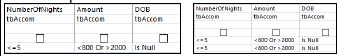
5.5
Only Name and Surname fields are displayed ✓
NumberOfNights criteria: <=5✓ (OR <6)
Amount field criteria: <800 ✓ OR ✓ >2000 ✓
DOB criteria: IS NULL OR Not Like "*"✓
AND operator for all field criteria ✓ (Note to marker: 2 records expected.)
1 1 3 1 1
7
Query: qry5_6
5.6
Calculated field: Discount:[Amount]-[Amount]*10/100 OR Discount:[Amount]-[Amount]*0.1 OR Discount:[Amount]*0.9 OR Discount:[Amount]*90/100
New calculated field Discount added ✓
10% calculated ✓
On the original Amount ✓
Subtract to get the difference ✓
1 1 1 1
4
Report: rpt5_7
5.7
Shading applied to Province field ✓ (in Province group header)
Amount field sorted ✓ in descending (largest to smallest) order
Function in Accommodation group footer/header ✓ =SUM ([Amount]) ✓ (Note to marker: Allocate the marks for the function even if it appears in the wrong place.)
1 1 1 2
5
Total for QUESTION 5
[40]
QUESTION 6 File name: 6Viti Total Q6: 20
NO marks should be allocated for answering this question using Word.
This question should be marked from the HTML code.
Numerical attribute values do not need to be in inverted commas.
A maximum of 1 mark will be deducted if one or more closing tags are omitted.
Closing tag(s) or triangular brackets omitted or incorrect nesting
-1
Total for QUESTION 6
[20]
QUESTION 7 File names: 7Calc, 7Rep Total Q7: 20
No.
Criteria
Maximum Mark
Candidate
Mark
7Calc: Num_Nom worksheet
7.1
Cell A3: RANDBETWEEN (100,999) OR =RAND()*(999-100)+100 OR =RANDBETWEEN(1,9)&RANDBETWEEN(0,9)& RANDBETWEEN(0,9)
RANDBETWEEN OR RAND function ✓
Lower boundary (Any 3-digit number) ✓
Upper boundary (Any 3-digit number) ✓ (Should be larger than lower boundary)
Cell B3: =LEFT(A3,1) OR TRUNC(A3/100) OR MID(A3,1,1) OR INT(A3/100) OR LEFT(A3)
LEFT function ✓ (OR TRUNC OR MID)
Extract one character from cell A3 ✓
Cell C3: =RIGHT(A3,1) OR MID(A3,3,1) OR MID(A3,LEN(A3),1) OR A3-INT(A3/10)*10 OR RIGHT(A3)
RIGHT function ✓ (OR MID)
Extract one character from cell A3 ✓
Cell D3: =IF(B3=C3,"YES","NO") OR =IF(EXACT(B3,C3),"YES","NO")
Check that B3=C3 ✓ (OR (B3<>C3))
Value if true: "YES" ✓
Value if false: "NO" ✓
1 1 1 1 1 1 1 1 1 1
10
7Calc: Vouch_Bewys worksheet
7.2.1
Cell E2: (Check for building blocks) =TODAY()<=DATE(YEAR(NOW()),MONTH(D2),DAY(D2)) OR =IF(TODAY()>=DATE(2017,MONTH(D2),DAY(D2)), "FALSE","TRUE") OR =IF(TODAY()<DATE(YEAR(TODAY()),MONTH(D2),DAY(D2)), "TRUE","FALSE") OR =IF(DATE(YEAR(TODAY()),MONTH(D2),DAY(D2))>=TODAY(),"TRUE", "FALSE") OR =OR(AND(MONTH(D2)=MONTH(TODAY()),DAY(D2) >=DAY(TODAY())),MONTH(D2)>MONTH(TODAY())) OR =OR(IF(MONTH(D2)>MONTH(TODAY()),TRUE), AND(MONTH(D2)=MONTH(TODAY()),DAY(D2) >=DAY(TODAY()))) OR =IF(MONTH(D2)>MONTH(TODAY()),"TRUE", IF(MONTH(D2)=MONTH(TODAY()),IF(DAY(D2) >=DAY(TODAY()),"TRUE","FALSE"),"FALSE"))
Criteria 1: Check if birth month is greater than current month ✓
Correct output (TRUE) if birth month/date is greater than current month/date ✓
Criteria 2: Check if current month is equal to birth month ✓ AND current day is greater or equal to birth day ✓
Correct output (TRUE) if both aspects in criteria 2 are true ✓
Correct output (FALSE) if criteria 2 is false ✓
Function copied to cells E3:E111 ✓ (Note to marker: Award the output mark if the second criteria is wrong but the output is correct.)